
Home > Improvement > Improvement Examples

When intuition, data and facts are united with the scientific method of problem solving, good things happen fast! Following are the key elements of a great Improvement Design:

TO FOLLOW


TO FOLLOW
TO FOLLOW
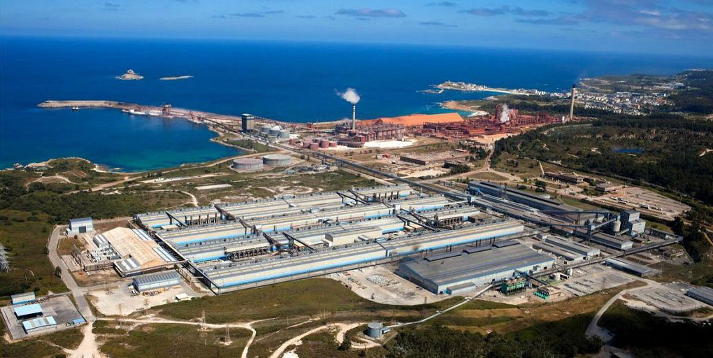
Figure 1 – Aluminum Plant in North of Spain
The General Manager of a large aluminum casting plant in the north of Spain was coached on how to develop a Strategic A3 for his operation. The GM used this one page A3 (Figure 2 below) as his “bible” for managing the business and kept it with him everywhere he went. He used the A3 to do checks on his team’s progress toward creating the Target State.
This is an excellent example on how a leader can develop a vision of where they want to take the business and then execute to build that vision. The GM was able to lead a major lean transformation, increasing capacity and reducing costs.
Improvement Metrics

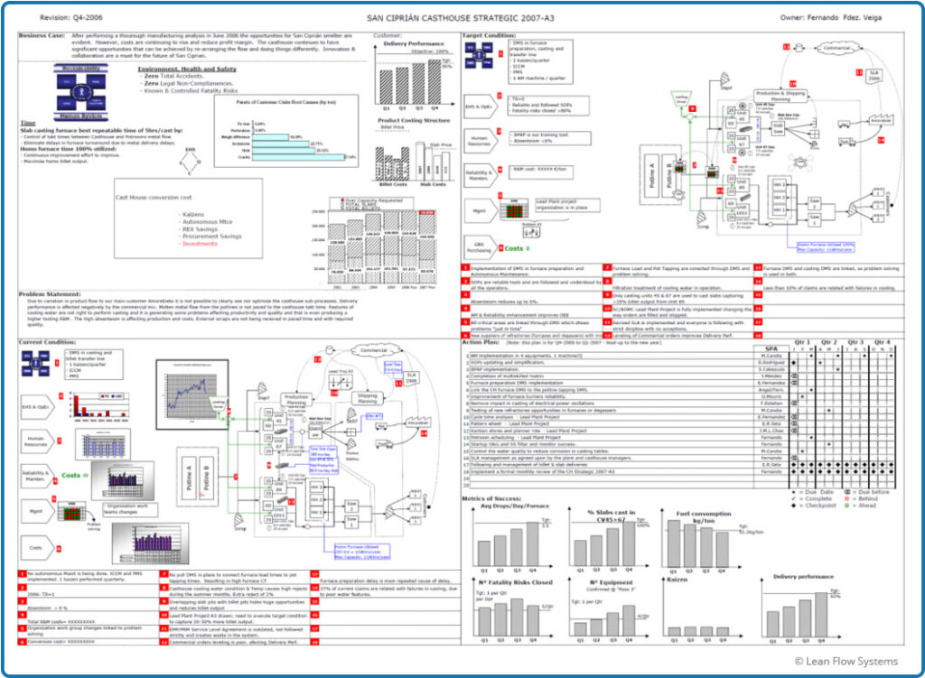
Figure 2 – Strategic A3 for Plant in Spain

Figure 1 – Borla Performance Exhaust Systems
We were asked to develop a proposal A3 for a client that makes aftermarket performance systems for the automotive industry. The client was struggling with complex flows, frequent reschedules and late shipments. We assessed the entire material and information flows and developed a target design that would simplify the operation.
The Current State required a deep dive into the products, plant layout and existing scheduling system. There were 45 different schedule signals, some of them conflicting with each other. This caused confusion and stress for the shop floor team as they tried to understand what to run from hour to hour.
The Target State features a complete, closed-loop Pull System with Heijunka Leveling. There is only one schedule for each flow path. Scheduling and inventory management would be visual on the shop floor and connect to Andons, thus facilitating clear visuals of what was needed to the entire operations team. Additionally, material flows are simplified, reducing material handling time and cost.

Figure 2 -Proposal A3 for Borla Performance Exhaust Systems
Flow Time Deep Dive

Background and Improvements
LFS had a three year engagement with a client to build a model lab (referred to as “Lab 0”) and cascade the improvements to an additional 20 labs. Toward the end of this engagement, we did a deep dive analysis of Lab 0, building a performance dashboard that compared before and after metrics for time, cost, quality and safety. We were pleased with improvements in labor productivity, where we saw improvements of 38% in one department and 192% in another department.
A critical time metric assessed was flow time. We concluded that average flow time was reduced 19%, flow time variability was reduced 34% and orders shipped in less than 5 days improved 9.8 percentage points (from 68.5% to 78.3%). While these results were good, we had expected bigger improvements in the neighborhood of 50% to 75%. This had been our experience with other businesses in the past. So we decided to look more closely to understand why the improvement hadn’t been better. This was our first objective for the data analysis:
Objective 1: Understand why flow time had not improved more.
Flow time is one of the most critical and under-calculated metrics in operations. While it’s relatively easy to get customer order lead time (typically calculated as Customer Receive Date/Time less Customer Order Date/Time), it can be very difficult to break lead time down by each process area. This kind of “under the hood” detailed analysis is critical to root cause problem-solving issues that cause order delays, wreck master schedules and anger customers. The second objective of the data analysis:
Objective #2: Illustrate the complexity of calculating detailed flow times with complex flows and inconsistently named product routing steps
Another confounding challenge with flow time is accurately measuring variability. Variability is one of the most corrosive waste drivers in a business so it’s important to measure it correctly. Histograms are a good start, but they are cumbersome to build and difficult to compare because you are contrasting graph shapes. It is better to fit a probability distribution function (pdf) to the data so more precise measures of scale (e.g. mean for Normal Distribution) and shape (e.g. Standard Deviation for Normal Distribution) can be done. The natural go-to pdf is the Normal (bell curve) distribution. The foundations of six sigma are based on this pdf. But is the data always Normal? If not, can it be made to be Normal? If the answers to these two questions are “no” and “no”, other pdf’s need to be assessed.
In the case of flow time, the data can be notoriously “anti-Normal”. Many factors cause flow time data to be irregular in shape: operator training and skill variability, machine reliability, change over time, material scheduling, its “non-zero nature” and product complexity, just to name a few. The third objective of the data analysis:
Objective #3: Show how to test a data set for normality and assess alternative pdf’s
What follows is a summary of the data analysis done on Lab 0 flow time to address the three objectives listed above.
Improvement Metrics
Flow Time Average Reduced 20%
Flow Time Variability Reduced 34%
Customer Experience
Orders Shipped <5 Days
Increased 9.8 Percentage Points
Mapping Out Flow Segments
The first step was to map out the major flow segments and figure out the Break Points where we wanted to capture the date and time for every order. These breakpoints were then used to calculate the flow times for major flow segments. For Lab 0 the breaks and flow time segments are shown in Figure 1. The lab is broken down into four departments: Surfacing, Coating, Finishing and Shipping. The goal was to calculate the Transfer Time, Queue Time and Department Flow Times. This was made very difficult for a number of reasons, for example:
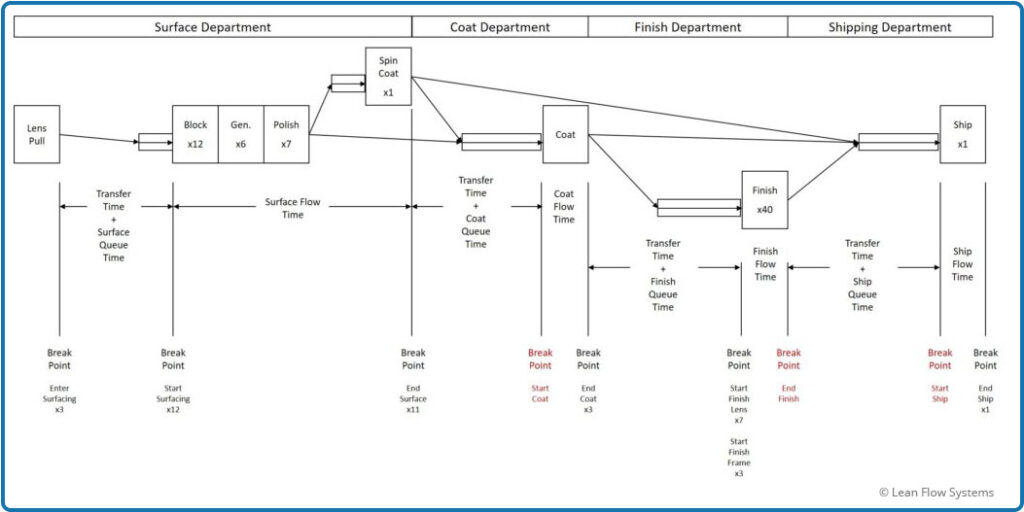
Figure 1 – Flow Time Break Points and Segments
Data Queries and Calculations
The complexities described in the previous section increased the number of queries and the complexity of the calculations by an order of magnitude. Figure 2 below shows the data mapping used to document the calculations. The boxes indicate Queries and Calculations. In total there were:
Figure 2 is shown only to underscore the need to simplify and standardize process flows and routing naming conventions.
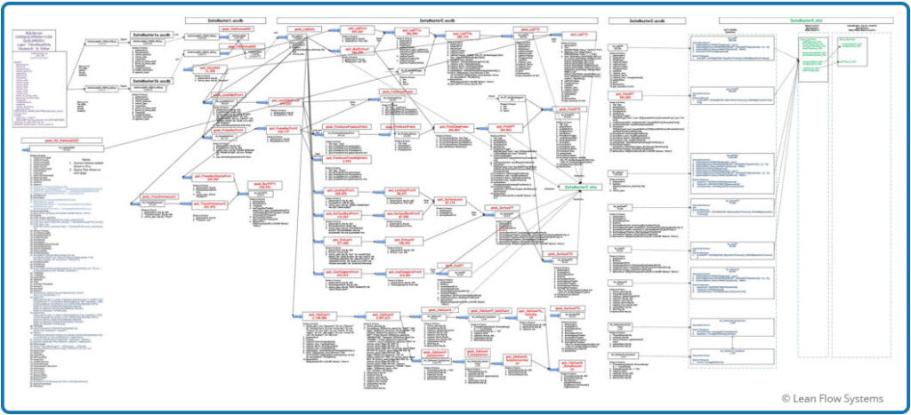
Figure 2 – Data Analysis Flow Diagram
Before and After Results
Figure 3 shows the average flow time and Figure 4 shows the average flow time plus 3 sigmas of variability, assuming a Normal pdf. We saw a 19% reduction in average flow time and a 34% reduction in the average plus 3 sigma. The way to interpret this is that, if the data is Normal, the worst flow time we would see for any order was 23.2 days before the initiative and 15.3 days after the initiative.
When we plot the Normal probability distribution function (pdf) curves for the Before and After data on the same chart we get a good visual of how the process has improved. The blue curve is the Before plot, the green curve is the After plot. Note how the curve stretches out longer to the right compared to the green After curve. This indicates that there are more jobs with longer flow times in the Before data set. Also, there is more area under the green curve to the left of the 5-day red line target. This indicates more jobs are getting done in less than five days.
Often we leave it at that and are happy with our results, feeling good about our assumption of Normality data. But is it safe to assume that the data are Normal? Often we plow right past this question because #1 the Normal pdf adequately covers many data sets, especially larger sets, and #2 it is quite convenient to talk about means and standard deviations with other people, it is a relatively easy concept to convey and has been socialized over the years. But for this example, we will take a deeper look at the data to see if this assumption is reasonable.
But one more question before doing all that work: why do we even care about matching an accurate pdf to the data? Why not just plot the data on a histogram and use that as our measure of performance? There are a few reasons we like to match pdf’s to data where possible:
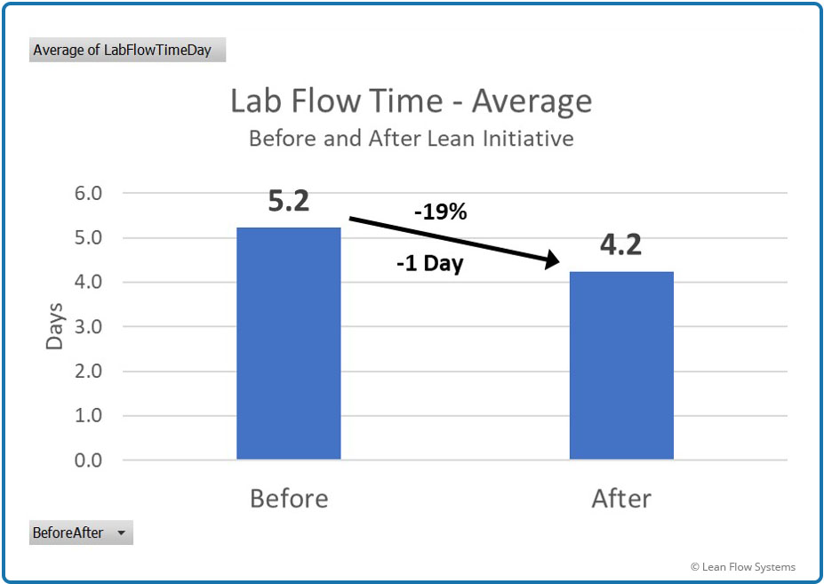
Figure 3
Average Flow Time
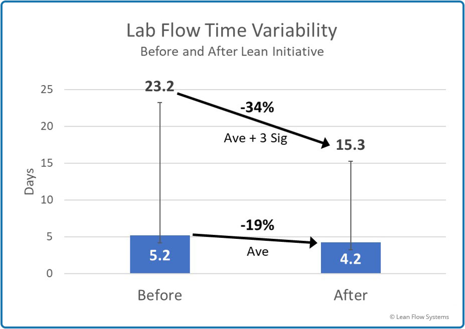
Figure 4
Average and Standard Deviation of Flow Time
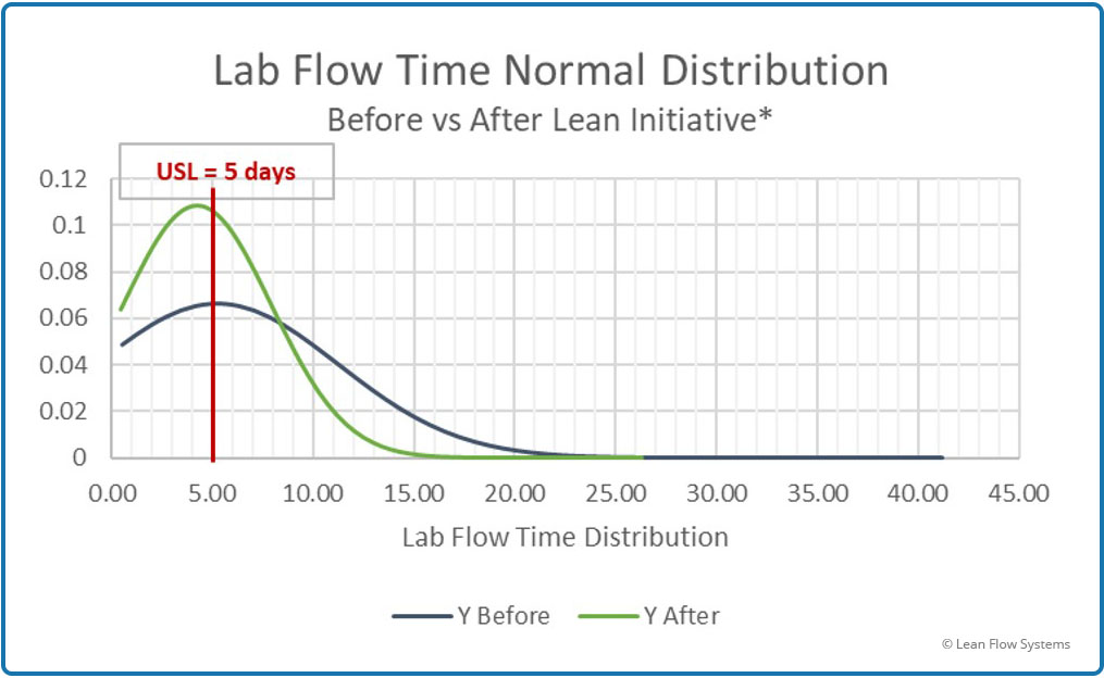
Figure 5 – Before and After Comparison of Normal pdf
Histogram Plots
Histogram plots are an excellent way to get a feel for how the data is shaped and how the process is behaving. Figures 6 and 7 show the histogram plots for the Before and After data sets. At first glance it is clear that the data points are clustering closer to the left of the graph for the After data, indicating that a greater proportion of jobs are getting done sooner. When we accumulate all the bars to the left of the 5 day line we arrive at the total percent of jobs getting done in less than 5 days: 68.5% Before, 78.3% After. However, the question still remains: is this data Normally distributed?
There are two aspects to the shape that indicate that the answer to this question is definitely “no”:
So we conclude, based on the subjective assessment of histogram shapes, the data is not Normal. Later in this analysis we will use some statistical tools to more objectively prove that this conclusion is correct. There are two options to consider at this point:
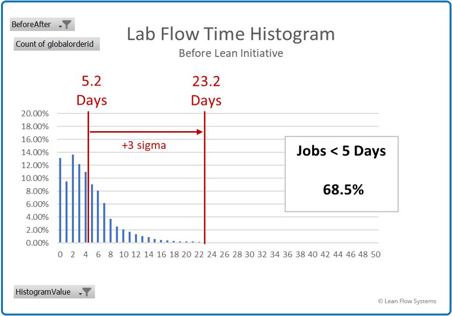
Figure 6 – Before Flow Time Histogram

Figure 7 – After Flow Time Histogram
Fitting Probability Density Functions to the Data
Figures 8 through 11 compare the actual histogram data to pdf estimates for four pdfs. Excel Solver was used to determine the Scale and Shape parameters for each pdf with the goal of minimizing the Chi-Square Cumulative Error. On each graph is a box indicating what percent of the jobs were predicted to be less than 5 days, what the actual number under 5 days were and the difference between these two numbers. Five days was selected because it was a key performance metric for the client.
A negative difference indicates that the pdf was conservative, meaning it predicted less jobs under 5 days than what actually occurred. A positive difference indicates that the pdf predicted more jobs to be less than 5 days than actual, thus an “optimistic” predictor. All things equal, we prefer conservative pdf’s to optimistic pdf’s because we don’t want to believe we are better than we actually are. Following are summaries of each pdf and a conclusion.
Before deciding on which pdf to use, we will test the data one more way. The Chi-Square Test (not to be confused with the Chi-Square pdf) accumulates the differences between each histogram bar and the pdf prediction for that bar for the entire data range, not just the <5 day test. The lower the total sum, the better the pdf fit. Following are the results of these tests for each pdf:
These errors match the histogram subjective conclusions.
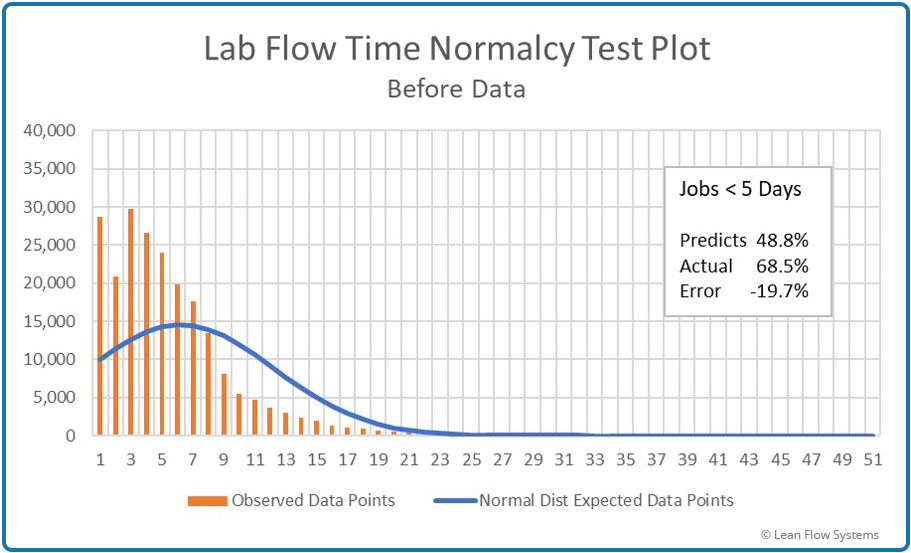
Figure 8 – Histogram vs Normal pdf
Under predicts by 19.7%
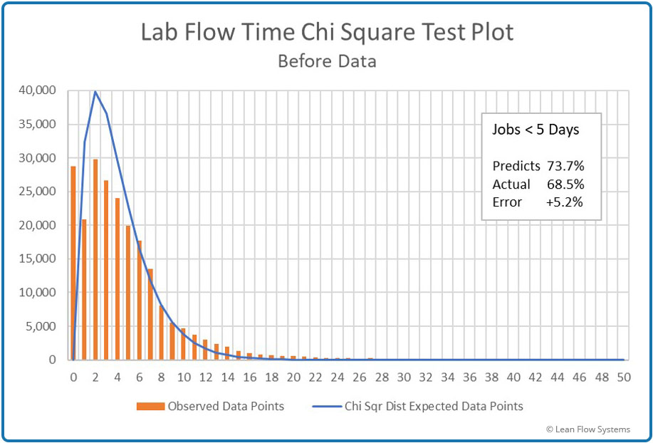
Figure 9 – Histogram vs Chi-Square pdf
Over predicts by 5.2%
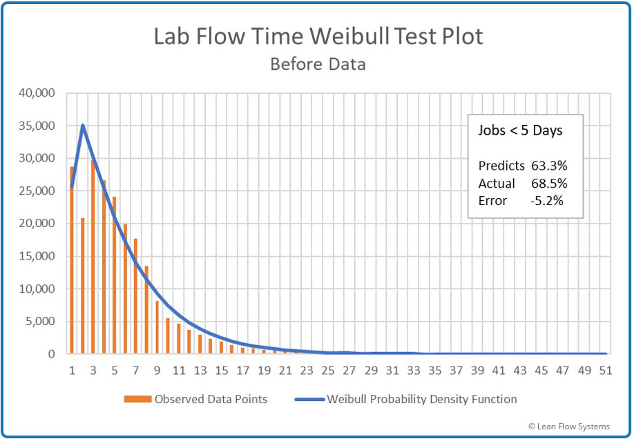
Figure 10 – Histogram vs Weibull pdf
Under predicts by 5.2%
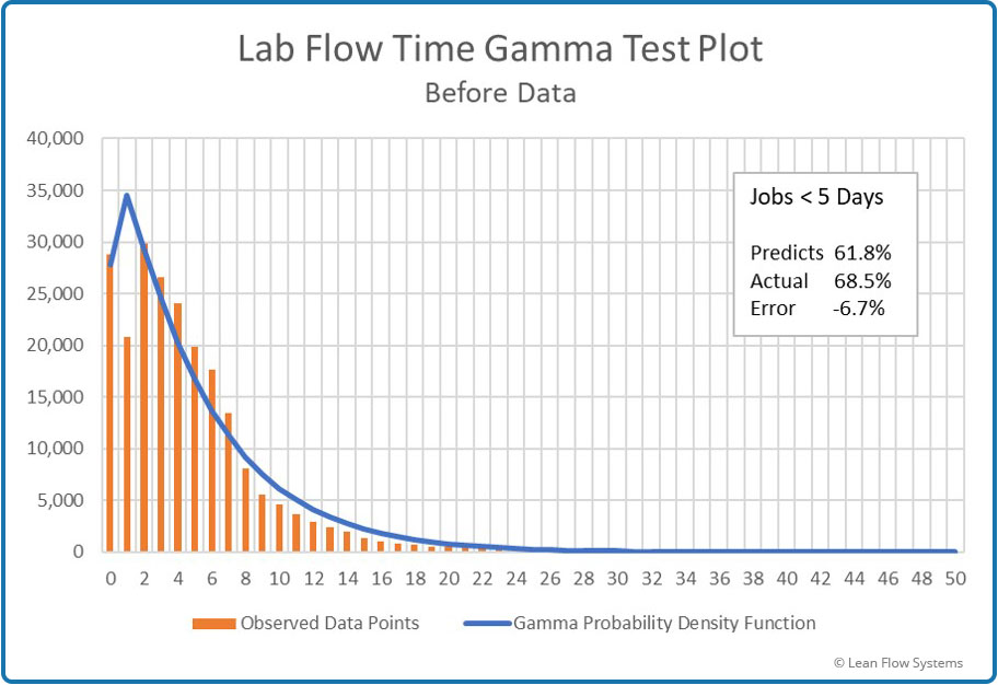
Figure 11 – Histogram vs Gamma pdf
Under predicts by 6.7%
While Weibull is more accurate at <5 days predictions, Gamma is the more accurate pdf for the entire data set (it has the lowest Cumulative Error). So, we pick Gamma. Now, let’s compare the Normal and Gamma pdf parameters to see the improvement in predictions of Scale and Shape, using the Before data:
Scale (Mean, or “Average”)
Normal: 5.2 Days
Gamma: 5.1 Days
Accuracy Improvement: 2%
Shape (Variance)
Normal: 35.9 days squared
Gamma: 5.5 days squared
Accuracy Improvement: 553% Improvement
So we see that there was a huge improvement in the accuracy of measuring variability. This is one of the key lessons of this analysis. Variability is a critical and very difficult metric to measure and reduce. It is one of the three core principles of the Toyota Production System:
Flow Time Variability Sources
As previously stated, we were disappointed in the 20% average flow time improvement. With all the work done and our past experience with other projects, we had expected a 50% to 75% improvement. Why the delta in expectation versus actual? We hypothesized that variability remained high and was dampening flow time improvements.
So what is causing all this variability? Following were our assumptions coming into the initiative, ranked by what we believed to be the highest to lowest impact:
We made great progress with 1, 2, 3 and 4. But the results for 5 were very disappointing. Breakage for lenses made internally by Lab 0 was flat, while breakage for lenses made at other labs (outsourced lenses) and sent to Lab 0 increased by 308%! Both these results were poor. This led us to look at the correlation between Breakage Count (how many times a job broke) and flow time. Figure 12 below is the graph of the Before and After data sets. There was an almost perfect correlation between the two, correlations coefficients of .99 and .94 for Before and After data, respectively.
This was a big learning for us. In conclusion, we had over-focused on points 1 through 4 and under-focused on point 5. This limited progress on flow time.

Figure 12 – Breakage/Flow Time Correlation

Background and Improvements
COMING SOON!